Supervised learning is the branch of machine learning behind spam filters, fraud detection systems, medical imaging tools, and large language models like ChatGPT. Understanding how it works, and where it reaches its limits, matters for anyone making decisions about building or buying AI-powered products.
What Supervised Learning Actually Is
Supervised learning is a method where a model learns from labeled examples, each pairing an input with the correct answer. A label is simply the known outcome: the sale price on a house that actually sold, the spam or not spam verdict on an email someone already classified, the “cat” or “dog” tag on an image a human annotated. The model studies those inputs and outputs, identifies the patterns connecting them, and applies those patterns to data it has never seen.
Supervised learning produces two types of outputs:
Classification asks the model to assign an input to one of a set of categories. Is this email spam or not? Will this loan applicant default? The answer is discrete.
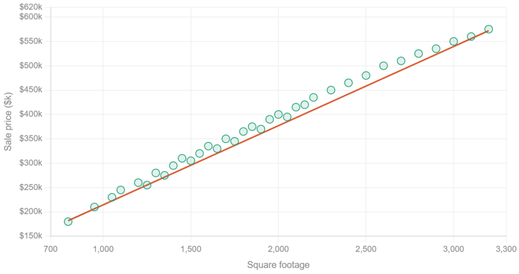
Regression asks the model to predict a continuous numerical value. What will this house sell for? How many inches of rain will fall tomorrow? The answer exists on a spectrum.
The Models Behind Supervised Learning
A model is the mechanism that learns from labeled data and makes predictions. Different problems call for different models, and the choice comes down to the type of output you need, the nature of your data, and how much complexity the problem actually requires.
Linear Regression predicts a continuous numerical value by finding the best-fit line through the training data. It works well when the relationship between inputs and output is relatively direct. A home price prediction model takes inputs like square footage, number of bedrooms, and location, and outputs an estimated sale price. The relationship between those inputs and price is direct enough that linear regression handles it without needing a more complex model.
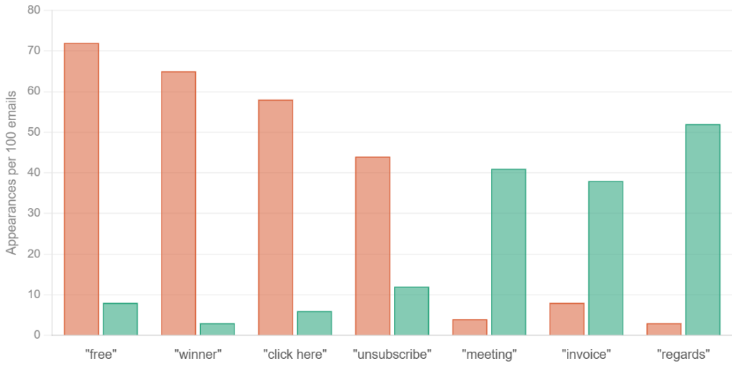
Naive Bayes is a classification model that calculates the probability that an input belongs to a category by counting how often each feature appears with each label in the training data. A spam filter is one of the earliest and most common applications. The model counts how often features like words and sender patterns appear in emails categorized as spam versus legitimate, then uses those frequencies to classify incoming messages. It trains fast and performs well with limited data, because it assumes each feature is independent of the others. For example, it assumes the word “free” appearing in an email has no bearing on whether “winner” also appears. That independence assumption is what earns it the “Naive” label: in practice, features often move together in meaningful ways. But the model works surprisingly well despite it and makes it a natural starting point for text classification problems.
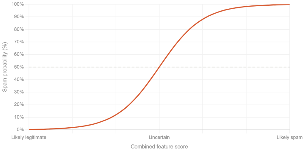
Logistic Regression is another classification model that outputs a probability. It works by assigning a weight to each input feature, where the weight represents how strongly that feature pushes the prediction toward one outcome or another. Applied to spam filtering, it takes the same inputs, words, sender patterns, header information, but assigns a weight to each one of these input features. That weight represents how strongly the feature pushes the prediction toward spam or legitimate. A high weight on the word “winner” means that word is a strong signal for spam. A negative weight on a recognized sender domain means the model pushes the prediction toward legitimate. Unlike Naive Bayes, logistic regression does not assume each feature acts independently of the others, which makes it more accurate when those features move together in ways that matter for the prediction.
Support Vector Machines (SVM) take a different approach to classification, one that becomes useful when categories don’t separate cleanly the way spam and legitimate email do. Consider classifying support tickets by type: billing, technical, account access. Naive Bayes counts how often each word appears in each category. Logistic Regression weights those words and draws a boundary between categories. Both approaches learn from every ticket in the training data.
SVM ignores most of the training data and focuses specifically on the tickets where the language is ambiguous enough that they could belong to more than one category. A ticket that says “I was charged for a plan I can’t access” contains language from two categories: “charged” points to billing, “can’t access” points to account access. SVM treats those ambiguous tickets as the most important signal for where to draw the line between categories and builds its classification rules around them rather than around the clear-cut cases.
You reach for SVM over Naive Bayes or Logistic Regression when your categories don’t separate cleanly and simpler models keep misclassifying the edge cases.
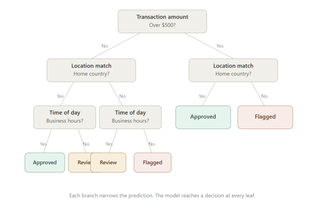
Decision Trees split data into branches based on input features, following a series of if-then rules until they reach a prediction. A credit card fraud detection model might first branch on transaction amount, then on whether the location matches the cardholder’s home country, then on time of day, ultimately outputting a decision: approve, flag for review, or block the transaction. Each branch narrows the prediction until the model reaches a conclusion. They are intuitive, easy to interpret, and handle mixed data types well. Their weakness is overfitting, where the model memorizes the training data rather than learning from it. A tree with enough branches does exactly that: it memorizes the fraud patterns it was trained on rather than learning rules that generalize to new ones.
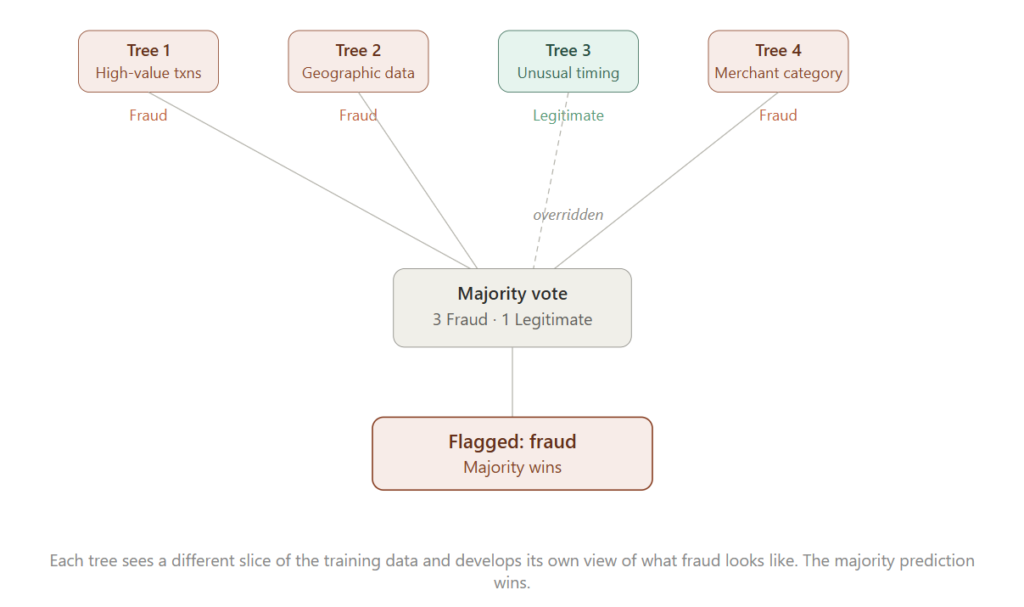
Random Forest addresses the overfitting problem in Decision Trees by building many trees instead of one. Each tree is trained on a different subset of the data, so no single tree sees the full picture. In credit card fraud detection, one tree might be trained heavily on high-value transactions, another on geographic anomalies, another on unusual timing, another on merchant category. Each tree develops a different view of what fraud looks like. When a new transaction arrives, all the trees vote, and the majority prediction wins. That diversity of perspectives makes the combined model generalize better than any single tree, which matters because fraud patterns constantly evolve.
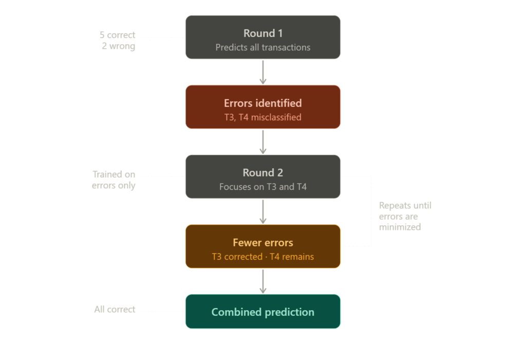
Gradient Boosting is another tree-based ensemble model, but it builds trees differently than Random Forest. Random Forest builds many trees independently and combines their votes. Gradient Boosting builds trees sequentially, where each tree focuses specifically on the cases the previous tree got wrong. In credit card fraud detection, the first tree makes predictions across all transactions. The second tree looks at where the first tree made errors and corrects them. Each subsequent tree corrects the errors of the one before it. The result is a model that improves iteratively rather than by averaging independent perspectives. XGBoost and LightGBM are the most widely used implementations. You reach for Gradient Boosting when you need high accuracy on tabular data and Random Forest isn’t getting you there.
Neural Networks process inputs through layers of interconnected nodes, where each layer learns to detect increasingly complex patterns. Consider predicting customer churn: whether a customer will cancel their subscription in the next 90 days. Logistic Regression approaches this by assigning a fixed weight to each input, login frequency, support ticket volume, account age, and combining them into a cancellation probability. It can account for interactions between signals, but only the ones an engineer explicitly builds in. If nobody thought to combine account age with login frequency, the model won’t catch that pattern. A neural network discovers those interactions on its own. The first layer asks what each signal is doing independently: is login frequency dropping? Are support tickets rising? The second layer asks what those observations mean when they happen together on the same account. A drop in login frequency combined with rising support tickets on a new account signals a higher cancellation risk than any of those signals alone, and the network learns that without an engineer defining it. Those combinations emerge from the data during training as the network adjusts the strength of connections between layers until its predictions match the known outcomes.
Convolutional Neural Networks (CNN) are a specialized type of neural network designed for image data. Rather than examining every pixel independently, they use filters that scan across the image to detect spatial features: edges, shapes, and textures in early layers, and increasingly complex structures in later layers. A chest X-ray fed into a CNN trained on thousands of labeled scans goes through the same process. Early layers detect edges and density variations in the tissue. Later layers combine those into patterns associated with conditions like pneumonia or malignant tumors. The output is a classification, a probability that the condition is present. The model is never told what pneumonia looks like. It learns to recognize the visual patterns associated with the condition from the labeled examples it was trained on.
Recurrent Neural Networks (RNN) and Long Short-Term Memory Networks (LSTM) are designed for sequential data where order matters. In speech recognition, the input is a stream of audio and the output is transcribed text. An RNN processes that audio one step at a time, carrying information forward from each step to the next. The problem is that over a long sequence, early context fades. By the time the model reaches the end of a long sentence, it may have lost track of how it started, which makes transcription unreliable. LSTMs solve this by deciding at each step what to remember and what to forget. A word like “not” early in a sentence changes the meaning of everything that follows. An LSTM learns to hold onto that word and carry its influence forward across the full length of the sentence.
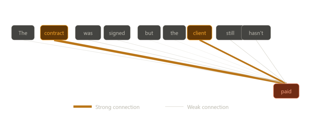
Transformers process entire sequences in parallel rather than step by step, which is what separates them from RNNs and LSTMs. An RNN works through a sentence one word at a time. A Transformer looks at every word simultaneously and weighs how relevant each word is to every other word in the sequence. In the sentence “The contract was signed but the client still hasn’t paid,” the word “paid” is more closely connected to “contract” and “client” than to “signed” or “but.” A Transformer learns those relationships across the full sequence at once rather than carrying them forward step by step. Large language models like ChatGPT are built on Transformers. The input is a sequence of words and the output is the next word in the sequence. That is also how the model is trained: given a sequence of words from a large body of text, predict the word that comes next. The label is the actual next word, derived from the text itself rather than assigned by a human. Doing that coherently across any topic, in any context, at any length is what makes Transformers the right architecture for the problem, and the reason these models require data and compute at a scale that puts them in a different category from everything else on this list.
Eight Examples at a Glance
The table below highlights 8 examples and maps their inputs, outputs, and the model typically used.
| Application | Input | Output | Model |
|---|---|---|---|
| Home Price Prediction | Property attributes | Estimated price | Linear Regression |
| Spam Filtering | Email content, sender data, header info | Spam / Not Spam | Naive Bayes / SVM |
| Fraud Detection | Transaction data, user behavior | Fraud / Not Fraud | Random Forest / Gradient Boosting |
| Customer Churn | Behavioral, transactional, demographic data | Churn probability | Logistic Regression / Neural Network |
| Document Classification | Text content | Category | SVM / Neural Network |
| Speech Recognition | Audio data | Transcribed text | RNN / LSTM |
| Medical Diagnosis | Medical imaging | Diagnosis / probability | CNN |
| ChatGPT / LLMs | Sequence of words | Next word prediction | Transformer |
Home price prediction is the most straightforward application in this group. The inputs are clean, the relationship between features and output is relatively direct, and a simple linear regression model handles it well. The four applications in the middle of the table, spam filtering, fraud detection, churn prediction, and document classification, require more work. You need a meaningful volume of labeled data, careful model selection, and ongoing maintenance as patterns shift over time, but they are manageable for teams with reasonable resources. Speech recognition and medical imaging sit above that. Both require large, specialized datasets and architectures purpose-built for their data types, and medical imaging in particular demands rigorous validation before any production use. Large language models are in a different category entirely. The data and compute required to train one from scratch puts that path out of reach for most organizations. That distinction matters when you are deciding whether to build a model internally, fine-tune an existing one, or use a third-party model through an API.
The next post in this series walks through building a spam filter from scratch, from defining the problem and assembling training data through model selection, labeling, training, and deployment.